Monitoring Classes
This chapter is supposed to give a quick overview over differences between the different implemented algorithms.
Conceptual basis
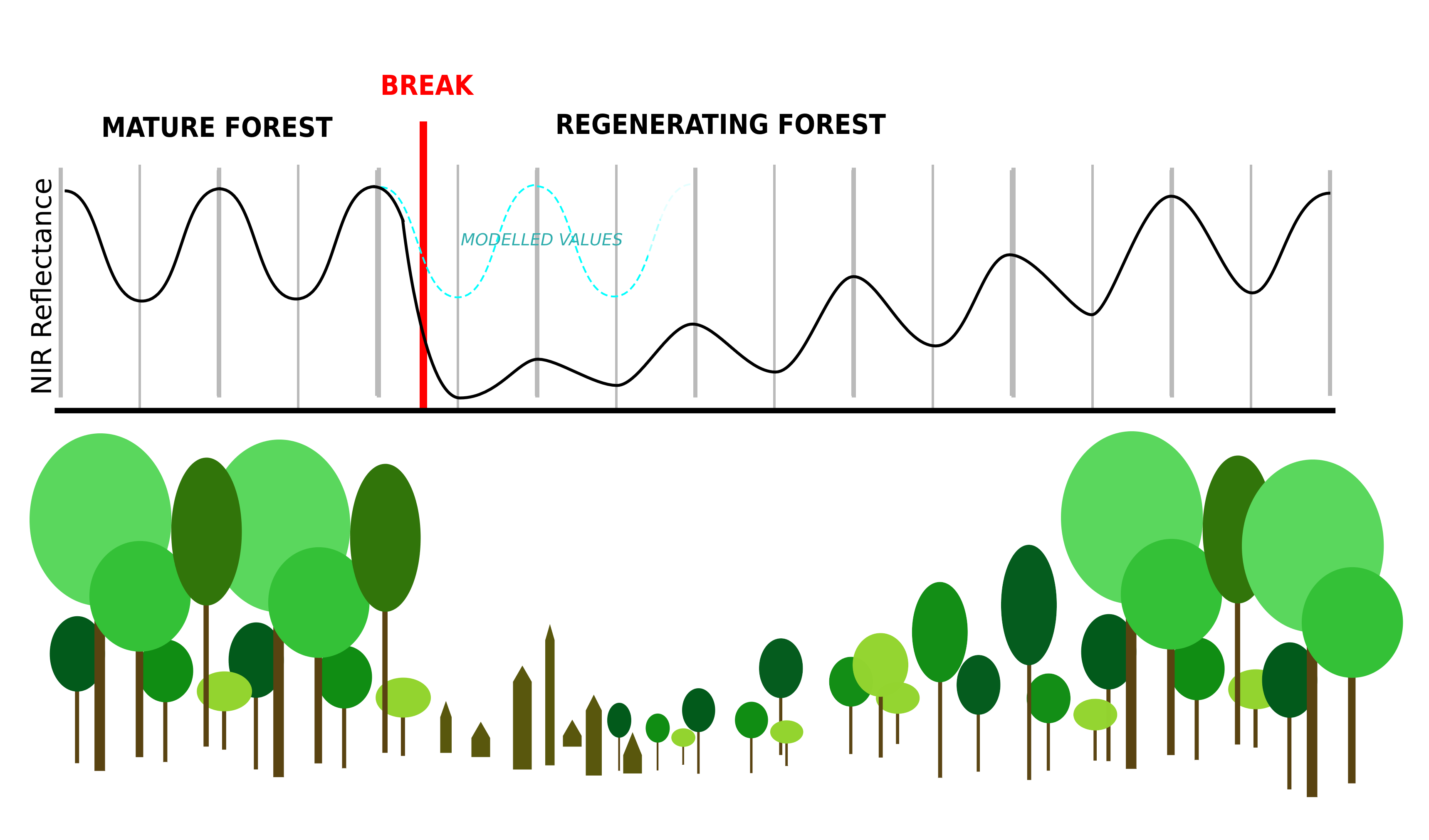
Conceptually, near real-time monitoring using time series analysis is based on the temporal signature of forests. Due to seasonal differences in leaf area, chlorophyll and other biophysical or biochemical attributes, vegetation dynamics can be visible in the spectral response of forests. As an example, healthy forests exhibit a high reflectivity in the Near Infrared (NIR) because of scattering in that wavelength caused by the structure and water content of the leaves. The number of leaves and thus of scattering in the NIR is highest in summer and spring and lowest during winter. This seasonal pattern can be modelled and used to detect disturbances.
© Copyright European Union, 2022; Jonas Viehweger
All implemented algorithms are based on this concept. They first fit a model to the stable forest, then monitor for unusual values compared to that model. How exactly this monitoring happens is one of the main differences between the algorithms.
EWMA
EWMA is short for exponentially weighted moving average and follows an algorithm as described by Brooks et al. (2013). This algorithm is based on quality control charts, namely Shewhart and EWMA quality control charts.
Instantiation
from nrt.monitor.ewma import EWMA

nrt_class = EWMA(trend=True, harmonic_order=2, mask=None,
                 sensitivity=2, lambda_=0.3, threshold_outlier=2)
This shows the parameters specific to the EWMA class in the second row during instantiating.
In particular this is sensitivity, lambda_ and threshold_outlier.
Let’s first talk about lambda_. Lambda (0<λ<=1) is used as the exponent for the
exponentially weighted moving average and basically controls how much influence the historic data has on the average.
So for a time series where \(x_t\) is the value at time period t, the EWMA value \(s\) at time t is given as:
First the value at time t is weighted by λ and then added to the previous EWMA value, which got weighted by the inverse of λ. That means, that for small λ the impact of single values on the average are low. So if the time series is very noisy, low values for lambda around 0.05 to 0.25 are recommended. This ensures that for example a single cloud which wasn’t masked doesn’t have a long lasting impact on the EWMA value.
The parameter sensitivity is used to calculate the process boundary (also called control limit)
which signals a disturbance when crossed.
The boundary is calculated as follows:
with CL as Control Limits, L as the sensitivity and \(\sigma\) as the standard deviation of the population. Basically the lower L is, the higher the sensitivity since the boundary will be lower. This is a very simplified formula since a few expectations are made. For a more detailed look at the formula, see the Wikipedia page.
Lastly threshold_outlier provides a way to reduce noise of the time series while monitoring.
It discards all residuals during monitoring which are larger than the standard
deviation of the residuals during fitting multiplied by threshold_outlier. This means that no disturbances which exhibit
consistently higher residuals than \(threshold \cdot \sigma`\) will signal, but it also means that most clouds
and cloud shadows which aren’t caught by masking will get handled during monitoring.
Fitting
By default EWMA is fit using OLS combined with outlier screening using Shewhart control charts. For more details see Fitting & Outlier Screening.
CCDC
CCDC is short for Continuous Change Detection and Classification and is described in Zhu & Woodcock (2014). The implementation in this package is not a strict implementation of the algorithm. It was also not validated against the original implementation.
There are a few main differences. In contrast to Zhu & Woodcock (2014), multivariate analysis is not available in the nrt package. Furthermore, due to the structure of the nrt package, the automatic re-fitting after a disturbance which is described in the original implementation is not available. Lastly, the focus of this package is the detection of breaks and not their classification, so this part of the original algorithm is also omitted.
Instantiation
from nrt.monitor.ccdc import CCDC

nrt_class = CCDC(trend=True, harmonic_order=2, mask=None,
                 sensitivity=3, boundary=3)
During instantiation, the two parameters sensitivity and boundary
influence how sensitive the monitoring with CCDC will be.
The parameter sensitivity in this case influences how high the threshold is after which
an observation will get flagged as a possible disturbance. This threshold also
depends on the residual mean square error (RMSE) which is calculated during fitting.
With CCDC everything which is higher than \(sensitivity \cdot RMSE\) is flagged as a possible
disturbance.
The boundary value then specifies, how many consecutive observations need to be above the threshold to confirm a disturbance.
So with the default values, during monitoring 3 consecutive observation need to be 3 times higher than the RMSE to confirm a break.
Fitting
By default CCDC is fit using a stable fitting method called CCDC-stable, combined
with outlier screening which is based on a robust iteratively reweighted least squares fit.
For more details see Fitting & Outlier Screening.
CuSum and MoSum
Monitoring with cumulative sums (CuSum) and moving sums (MoSum) is based on Verbesselt et al. (2013) and more particularly the bfast and strucchange R packages.
Both algorithms have the same underlying principle. The assumption is, that if a model was fitted on a time-series of a stable forest, the residuals will have a mean of 0. So summing all residuals up, the value should stay close to zero. If however then a disturbance happens, the residuals will consistently be higher or lower than zero, thus gradually moving the sum of residuals away from 0.
The major difference between the two algorithms is that CuSum always takes the cumulative sum of the entire time-series, while MoSum only takes the sum of a moving window with a certain size.
Instantiation
CuSum
from nrt.monitor.cusum import CuSum

nrt_class = CuSum(trend=True, harmonic_order=2, mask=None,
                  sensitivity=0.05)
The parameter sensitivity in the case of CuSum and MoSum is equivalent to the significance level of the disturbance event.
It basically signifies how likely it was, that the threshold was crossed randomly and not caused by a structural change
in the time-series.
So in this case lower values decrease the sensitivity of the monitoring to structural changes.
MoSum
from nrt.monitor.mosum import MoSum

nrt_class = MoSum(trend=True, harmonic_order=2, mask=None,
                  sensitivity=0.05, h=0.25)
The only additional parameter in MoSum is h, which sets the moving window size relative to the
the total number of observations which were used during fitting. So if during fitting 40 observations
were used, with h=0.25 the window size during monitoring will be 10 observations.
Note
Since the process boundary during monitoring is pre-computed only for select values of sensitivity and h,
only 0.25, 0.5 and 1 are available for h and sensitivity has to be between 0.001 and 0.05
Fitting
By default CuSum and MoSum use a reverse ordered cumulative sum (ROC) to fit a stable period.
For more details see Fitting & Outlier Screening.
IQR
IQR is an unpublished experimental monitoring algorithm based on the interquartile range of residuals.
Instantiation
from nrt.monitor.iqr import IQR

nrt_class = IQR(trend=False, harmonic_order=3, mask=None,
                sensitivity=1.5, boundary=3)
The flagging of residuals works similar to CCDC.
The parameter sensitivity in this case influences how high the threshold is after which
an observation will get flagged as a possible disturbance. This threshold also
depends on the IQR as well as the 25th and 75th percentile which are calculated during fitting.
With this monitor everything which is higher than
\(q75 + sensitivity \cdot IQR\) or lower than \(q25 - sensitivity \cdot IQR\)
is flagged as a possible disturbance.
The boundary value then specifies, how many consecutive observations need to be above the threshold to confirm a disturbance.
Fitting
By default IQR is using an OLS fit.
For more details see Fitting & Outlier Screening