STAC monitoring pipeline

Run a monitoring simulation anywhere in the world using STAC

This example demonstrates how to retrieve satellite image time-series from a cloud archive, given a pair of coordinates anywhere in the world, and use them for a monitoring simulation. Here, “simulation” does not refer to simulated data; the example uses real data to detect actual land dynamics. The term highlights the retrospective nature of the exercise, distinguishing it from real-time monitoring systems. For this example, data is retrieved from the Microsoft Planetary Computer archive, which is indexed in a Spatio-Temporal Asset Catalogue (STAC), making it queryable in an interoperable way. While querying and preparing data extends slightly beyond the nrt package’s scope, we aim to provide a comprehensive view of the entire pipeline. Specifically, this example demonstrates how to:

• Query Landsat Collection 2 data for any location using the Planetary Computer STAC catalogue

• Load a datacube as an in-memory xarray dataset using odc-stac and dask

• Prepare the Landsat data for further analysis (mask clouds and shadows, apply scaling and offset, compute vegetation indices)

• Generate a simple rule-based forest mask

• Simulate a near real-time monitoring scenario

# sphinx_gallery_thumbnail_path = '_static/iqr_results_bolivia.png'

Define the study area

Here we prepare a bounding box of 20 by 20 km, centered on a forest area near the city of Concepción in Bolivia (The area is further described in [1]). Center coordinates are in longitude, latitude which is the Coordinate Reference System we generally get from most online services (google maps or simply typing “name of the place coordinates” in a search engine). To expand these coordinates to a bounding box of 20 km side, we transform the center point to a metric equidistant custom CRS (local UTM, if known could be used as well) and expand the point. Because the STAC API, later used to query the data, expects a bounding box with coordinates in EPSG:4326, we convert the bbox back to that CRS.

from shapely.geometry import Point
from shapely.ops import transform
from pyproj import CRS, Transformer

# Define centroid as a shapely point (in EPSG:4326)
centroid = Point(-61.725, -16.162)
# Custom equidistant CRS centered on the centroid
local_crs = CRS(proj='aeqd', datum='WGS84', lat_0=centroid.y, lon_0=centroid.x)
transformer = Transformer.from_crs(CRS.from_epsg(4326), local_crs, always_xy=True)
# Transform centroid to custom CRS, expand to bbox and transform back to EPSG:4326
centroid_proj = transform(transformer.transform, centroid)
bbox_proj = centroid_proj.buffer(10000).bounds
bbox = transformer.transform_bounds(*bbox_proj, direction='INVERSE')

Query and load the data

Here we query 5 years of Landsat data that intersect the previously defined study area. pystac-client is used to handle the query, while we use odc-stac in combination with dask to efficiently load the data as an xarray.Dataset. The local Dask cluster allows loading data in parallel, which can speed up the overall process. However, the main bottleneck here is network speed, and parallelization may not be very advantageous on a slow network, particularly for this example, which does not perform any data warping.

The resulting Dataset has the following dimensions (y: 671, x: 672, time: 67) and contains four data variables (red, nir08, swir22 and qa_pixel).

import datetime

import xarray as xr
import numpy as np
from pystac_client import Client as psClient # psClient to not be confused with dask's Client
from odc.stac import stac_load, configure_rio
from dask.distributed import Client, LocalCluster
import planetary_computer as pc


# Set up a local dask cluster and configure stac-odc to efficiently deal with cloud hosted data
# while taking advantage of the dask cluster
# Different types of configuration will be re
cluster = LocalCluster(n_workers=5, threads_per_worker=2)
client = Client(cluster)
configure_rio(cloud_defaults=True, client=client)


# Open catalogue connection and query data
date_range = [datetime.datetime(2017,1,1), datetime.datetime(2021,12,31)]
catalog = psClient.open('https://planetarycomputer.microsoft.com/api/stac/v1',
                        modifier=pc.sign_inplace)
# Query all Landsat 8 and 9 that instersect the spatio-temporal extent and have a
# scene level cloud cover < 50%
query = catalog.search(collections=["landsat-c2-l2"],
                       bbox=bbox,
                       datetime=date_range,
                       query={"eo:cloud_cover": {"lt": 50},
                              "platform": {"in": ["landsat-8", "landsat-9"]}})

# Load the required bands as a lazy (dask based) Dataset
ds = stac_load(query.items(),
               bands=['red', 'nir08', 'swir22', 'qa_pixel'],
               groupby='solar_day',
               chunks={'time': 1},
               bbox=bbox,
               patch_url=pc.sign,
               fail_on_error=False)

# Trigger computation to bring the data in memory (depending on network speed, this step may
# take up to a few minutes)
ds = ds.compute()
ds

<xarray.Dataset>
Dimensions:      (y: 671, x: 672, time: 67)
Coordinates:
  * y            (y) float64 -1.777e+06 -1.777e+06 ... -1.797e+06 -1.797e+06
  * x            (x) float64 6.262e+05 6.263e+05 ... 6.464e+05 6.464e+05
    spatial_ref  int32 32620
  * time         (time) datetime64[ns] 2017-01-28T14:10:25.141063 ... 2021-11...
Data variables:
    red          (time, y, x) uint16 7922 7918 7960 7946 ... 8766 8802 8588 8453
    nir08        (time, y, x) uint16 19040 18943 19307 ... 19187 20724 22073
    swir22       (time, y, x) uint16 9048 9042 9069 9116 ... 10815 10658 10374
    qa_pixel     (time, y, x) uint16 21824 21824 21824 ... 21824 21824 21824

Data Preparation

Data preparation involves three primary steps:

• Masking the Data: Use the qa_pixel layer to mask pixels contaminated by clouds and shadows. Observations classified as “invalid” due to cloud or shadow coverage are converted to np.nan to signify missing data.

• Applying Scale and Offset: Adjust the raw satellite data by applying necessary scaling factors and offsets to convert pixel values into calibrated surface reflectance values.

• Computing Vegetation Indices: Compute the Normalized Difference Vegetation Index (NDVI) which will be used later on in the monitoring process

Cloud Masking

Each Landsat scene includes a qa_pixel layer that provides bit-encoded Quality Assurance flags. This method of encoding uses bits to represent different conditions such as cloud, cloud shadow, and snow, allowing a vast range of scenarios to be compactly represented without the need for an extensive table of correspondences. This bit encoding approach, while efficient, makes interpreting mask values less intuitive compared to simpler methods like the Sentinel-2 SCL mask, which uses mutually exclusive integers to classify conditions.

According to the Landsat Collection 2 Product Guide on page 13, conditions such as fill, dilated cloud, cirrus, cloud, and cloud shadow are encoded into bits 0, 1, 2, 3, and 4, respectively. In temperate regions, it might also be necessary to mask snow, although it is generally not a concern for areas without snow coverage. The bit mask for these conditions is 0001 1111, which is more conveniently represented in hexadecimal as 0x1F. Pixels in the qa_pixel layer that have any of these bits set will return non-zero values when processed with np.bitwise_and and the mask 0x1F.

Scale and offset

Still according to the product guide (p.12), a scale and an offset must be applied to each band to obtain surface reflectance.

Warning

Note that the presence of the offset makes this step absolutely necessary, even when working with ratios or normalized indices such as the NDVI. In the past many satellite datasets only had a scaling factor but no offset, making it possible to work directly on raw data.

# Compute binary mask
mask = np.bitwise_and(ds.qa_pixel.values, 0x1F) == 0
# Convert invalid pixels to np.nan and drop qa_pixel
ds_clean = ds.where(mask).drop_vars('qa_pixel')
# Apply scaling and offset
ds_clean = ds_clean * 0.0000275 - 0.2
# Compute NDVI
ds_clean['ndvi'] = (ds_clean.nir08 - ds_clean.red) / (ds_clean.nir08 + ds_clean.red)

# Split the dataset into history and monitoring period
history = ds_clean.sel(time=slice(datetime.datetime(2017,1,1),
                                  datetime.datetime(2019,12,31))) # 3 years
monitor = ds_clean.sel(time=slice(datetime.datetime(2020, 1, 1), None))

Forest mask

It is generally recommanded, for more targetted monitoring, to provide a forest mask during instantiation of one of the nrt.monitor classes. There are many ways to obtain a forest mask, such as using global products or from a custom local classification. Here we use a rule based approach proposed by Zhu et al. (2012) as part of an article on continuous forest disturbances mapping [2]. The reasoning of that rule based algorithm is that forests have a high NDVI (high “greenesss”) and are relatively “dark” in the short wave infrared part of the light sprectrum. The long term NDVI and SWIR values both correspond to the intersect of a temporal regression with a single annual harmonic component. The following rule can then be used to distinguish forested from non-forested land.

IF beta0_NDVI > 0.6 AND beta0_SWIR2 < 0.1:
    pixel = Forest
ELSE:
    pixel = non-Forest

Intersect thresholds of 0.6 and 0.1 are those used in Zhu et al. (2012) and were defined for termporate forests in the United States of America. Here, we are in semi-deciduous context and forests are likely “greener” overall. We therefore adjusted the thresholds to exclude as many non-forested pixels as possible from the forest mask.

To quickly compute these long term NDVI and SWIR intersects in a non-verbose way, we can (mis)use the private ._fit method present in all nrt.monitor classes.

from nrt.monitor.iqr import IQR
import matplotlib.pyplot as plt
from matplotlib.colors import ListedColormap
from matplotlib_scalebar.scalebar import ScaleBar

# Prepare matrix of regressors
X = IQR.build_design_matrix(dataarray=history.ndvi,
                            trend=False, harmonic_order=1)
# Instantiate an arbitrary class from nrt.monitor
iqr = IQR()
# Use _fit to get beta arrays
beta_ndvi, _ = iqr._fit(X, history.ndvi)
beta_swir, _ = iqr._fit(X, history.swir22)
# Apply logical rule (first 'layer' of beta arrays is the intersect)
# Thresholds adjusted to be more restrictive
forest = np.logical_and(beta_ndvi[0] > 0.7, beta_swir[0] < 0.09).astype(np.uint8)

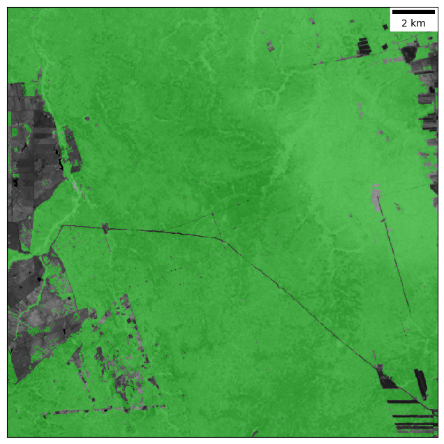
# Visualize
forest_cmap = ListedColormap([(0, 0, 0, 0), (0, 1, 0, 0.4)])
scalebar = ScaleBar(30)
plt.figure(figsize=(8, 8))
plt.imshow(history.ndvi[21], cmap='gray', interpolation='none',
           vmin=0.2, vmax=1.3)
plt.imshow(forest, cmap=forest_cmap, interpolation='none')
ax = plt.gca()
ax.add_artist(scalebar)
ax.set_xticks([])
ax.set_yticks([])

Monitoring simulation

In this section, we simulate near real-time monitoring by using three years of historical data for model fitting, followed by monitoring over a two-year period. Here are key details about the chosen monitoring algorithm and parameters:

• Monitoring Algorithm: We chose the Inter-Quantile Range (IQR) algorithm. This simple method counts consecutive anomalies to confirm a disturbance, making it effective for detecting abrupt changes like deforestation in environments with high natural variability. It is sensitive enough to pick up real disturbances without being falsely triggered by occasional extreme conditions, such as a particularly dry dry-season that temporarilly causes large regional drops in greeness.

• Baseline Model: We used a robust fitting method (RIRLS) to establish the baseline model. This technique reduces the influence of outliers, such as an extreme drought year in the historical data, ensuring the model is stable.

# Instantiate IQR class
model = IQR(mask=forest,
            harmonic_order=1,
            trend=False,
            sensitivity=1.4,
            boundary=4)
# Fit temporal model over stable history period
model.fit(dataarray=history.ndvi, method='RIRLS', maxiter=5)

# Run .monitor on each observation of the monitoring period, one at the time
for date in monitor.time.values.astype('M8[s]').astype(datetime.datetime):
    ds_sub = monitor.sel(indexers={'time': date}, method='nearest')
    model.monitor(array=ds_sub.ndvi.values, date=date)

# Visualize
mask_cmap = ListedColormap([(0, 0, 0, 0),
                            (0, 1, 0, 0.1),
                            (1, 0, 0, 0.1),
                            (1, 0, 1, 0.4)])
scalebar = ScaleBar(30)
plt.figure(figsize=(8, 8))
plt.imshow(ds_clean.ndvi[60], cmap='gray', interpolation='none',
           vmin=0.2, vmax=1.3)
plt.imshow(model.mask, cmap=mask_cmap, interpolation='none')
ax = plt.gca()
ax.add_artist(scalebar)
ax.set_xticks([])
ax.set_yticks([])

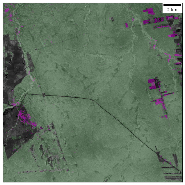
The resulting mask reveals clear signs of agricultural expansion in the east and south-west of the study area, as well as more subtle traces of selective logging in the north. Patterns in the north-west corner are likely errors due to unexpected natural variability.

References

[1]

Dutrieux, L.P., Verbesselt, J., Kooistra, L., & Herold, M., 2015. Monitoring forest cover loss using multiple data streams, a case study of a tropical dry forest in Bolivia. ISPRS Journal of Photogrammetry and Remote Sensing, 107, pp.112-125. https://doi.org/10.1016/j.isprsjprs.2015.03.015

[2]

Zhu, Z., Woodcock, C.E. and Olofsson, P., 2012. Continuous monitoring of forest disturbance using all available Landsat imagery. Remote sensing of environment, 122, pp.75-91. https://doi.org/10.1016/j.rse.2011.10.030